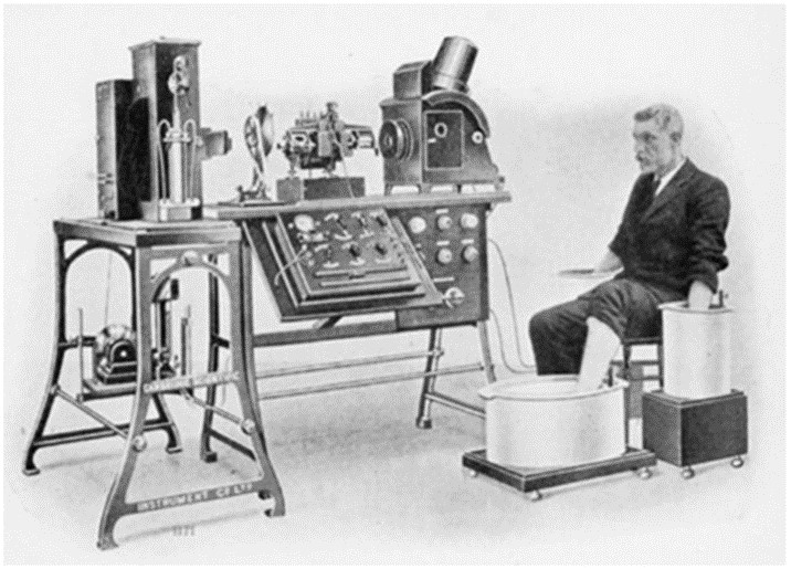
Willem Einthoven, professor in Leyden, invented the string galvanometer (in 1901), that was more sensitive and fast responding compared to the previous galvanometers. He was a physiologist who also worked with patients, and he was rewarded by a Nobel prize in medicine in 1924 for his work on ECG.
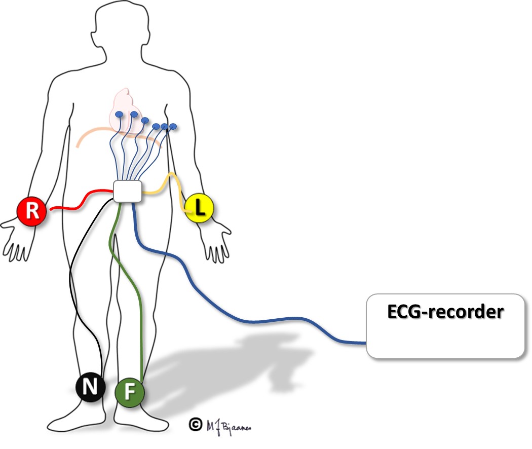
The body is a good conductor, so cardiac currents can be recorded from the surface. Patients’ arms and a foot were placed into buckets with saline, and the galvanometer measured the potential difference between the buckets (see picture). The patient must be relaxed (ideally not even talking), since all muscle activity generates electrical current, and we want to study cardiac activity with a minimum of electrical noise. The position of the heart within the thorax varies a little, depending on the body position. Optimal standardization of the recording is important for comparison with normal values, and registration from the supine patient is thus optimal.
Willem Einthoven and a patient ready for ECG recording (from Wikipedia)
The electrodes should be attached to smooth skin; hairy skin should be shaved. Conductive pads which are attached to the skin, enable recording of electrical currents. A conducting gel soaks the skin and reduces resistance. The adhesive must provide a stable skin contact, but also be non-irritating and easily removed. Old dry pads adhere poorly and cause noisy signals. The electrodes must be placed accurately at their recommended positions, and the cables should not be twisted, coiled or allowed to move during recording to avoid noisy signals.
The ECG deflection
The depolarizing wave front, by definition, determines the direction of the galvanometer response: a depolarizing wave front that moves toward the anode, is expressed as an upward (positive) deflection, whereas movement away from the anode is downward (negative), and a perpendicular wave front will be presented either as a flat line or as equal positive and negative components (see the figure below).
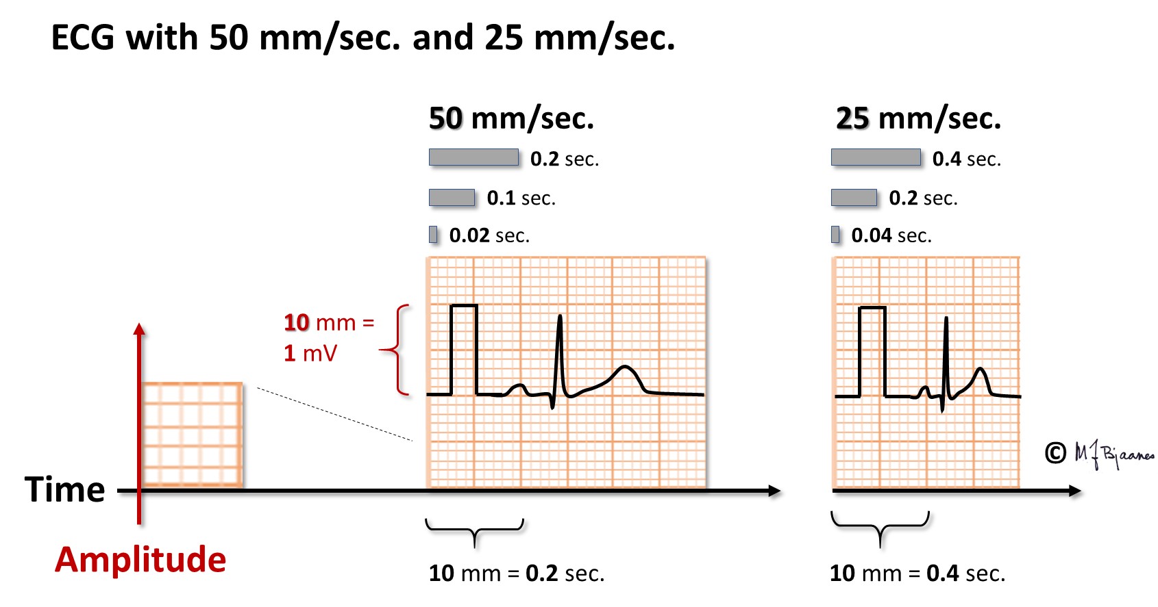
The voltage difference determines the height of the deflection (the amplitude). With a standard gain of 10 mm/mV, each mm represents 0.1 mV.
The duration of the impulse determines the width of the deflection. With a recording speed of 50 mm/s, 1 mm reflects 20 milliseconds.


The electrodes each have their defined position on the skin, and monitor local voltage changes. There are, however, many sources of errors:
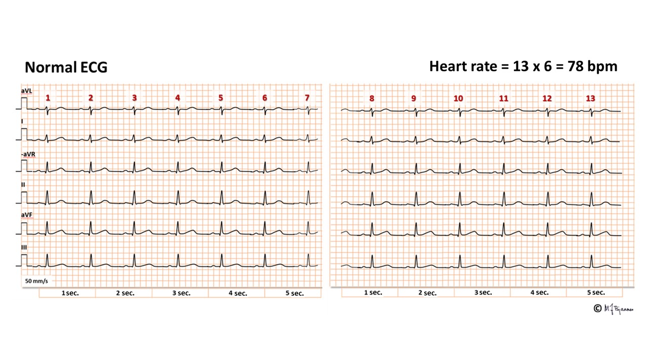
Optimally, the ECG is presented on graph paper. This facilitates measurements of amplitudes and time intervals. In the Nordic countries a paper speed of 50 mm/s is usually preferred because time intervals then can be more accurately measured (important for q waves, qR and QRS duration). The paper speed of 25 mm/s, commonly used elsewere, presents more heart beats per sheet. At the paper speed of 50 mm/s, a 1 mm square represents 1/50 s, i.e. 20 ms, and a larger, 5 x 5 mm square covers 0,1 s (100 ms) and 5 cm (50 mm) of course 1 second.
Heart rate can be calculated in several ways:
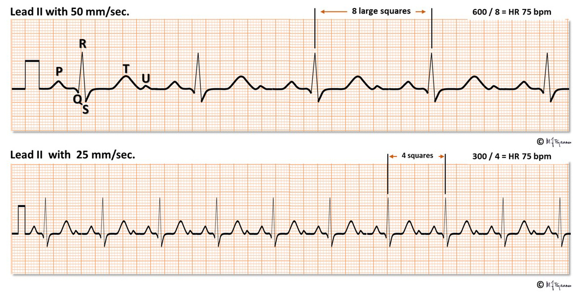
The standard presentation is 10 mm amplitude for 1 mV voltage, usually written on the print out or shown by a rectangular signal at the front of each channel (see on the left side of the above illustration). If amplitudes are huge and overlap, 5 mm/mV may be used, and very small amplitudes may be augmented to 20 mm/mV.
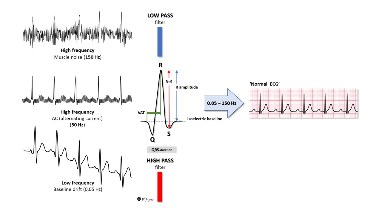
Aim: To obtain representative cardiac signals with minimal disturbance from alternating current noise, other muscles or respiration. The frequency band of interest is between 0.05 and 150 Hertz. The QRS signals are mainly high frequency (10-100 Hz), whereas ST (0.05-10 Hz) and the T wave are lower (1-2 Hz).
AC current may cause continuous noise. The apparatus is therefore equipped with a 50 Hz (or 60 Hz, if appropriate) «stop filter». A «high pass filter» removes the disturbing low frequency signals from respiration, body movements and other causes of baseline drifting, but if the threshold is too high, the ST segment will be distorted, interfering with detection of ischemia. The “low-pass filter” removes high frequency noise from striated muscle, but if set too low (by use of the muscle noise filter with threshold 30-40 Hz), important components of the QRS signal are lost (amplitudes are reduced and fragmented signals are “normalized”).
For a resting ECG the person should lie down relaxed with calm, slightly superficial respiration, and standard filter setting 0.05-150 Hz. This provides nice and representative signals. For exercise ECG electrodes are placed on the body to reduce noise from extremity muscles and the low-pass muscle noise filter (30-40 Hz) is activated. The 20% or so loss of QRS amplitude is then acceptable since the purpose is to detect possible ischemia as evidenced by STT changes, and arrhythmias. For long-term ECG (Holter ECG) the sampling window is narrow: a low setting of the low- pass filter reduces muscle noise, and a high threshold for the high pass filter reduces the noise from movements. Despite this, distinct P and QRS waves are usually recorded, allowing analysis of rate and rhythm. To avoid noisy, ugly ECG recordings, it may be tempting always to use the 35 Hz noise filter, but that may reduce the quality of the interpretation.
DO NOT USE THE MUSCLE NOISE FILTER WHEN RECORDING RESTING ECG!First, place the 10 electrode pads according to guidelines:
Now the cables should be connected. Established routines reduce risk of error, so always use the same sequence:
The chest leads (precordials) are frequently erroneous placed, leading to incorrect interpretation.
These were Einthoven’s three original leads, and he presented them as a triangle. Each lead presents the electrical activity of the heart, as seen from different viewpoints in the frontal plane (as we look at the heart from the front or back side). The leads may also be presented in a clock or compass format: The first lead (I) er 0° (east, 3 o’clock), the second (II) 60° (south-southeast, 5 o’clock) and the third (III) 120° (south-southwest, 7 o’clock).

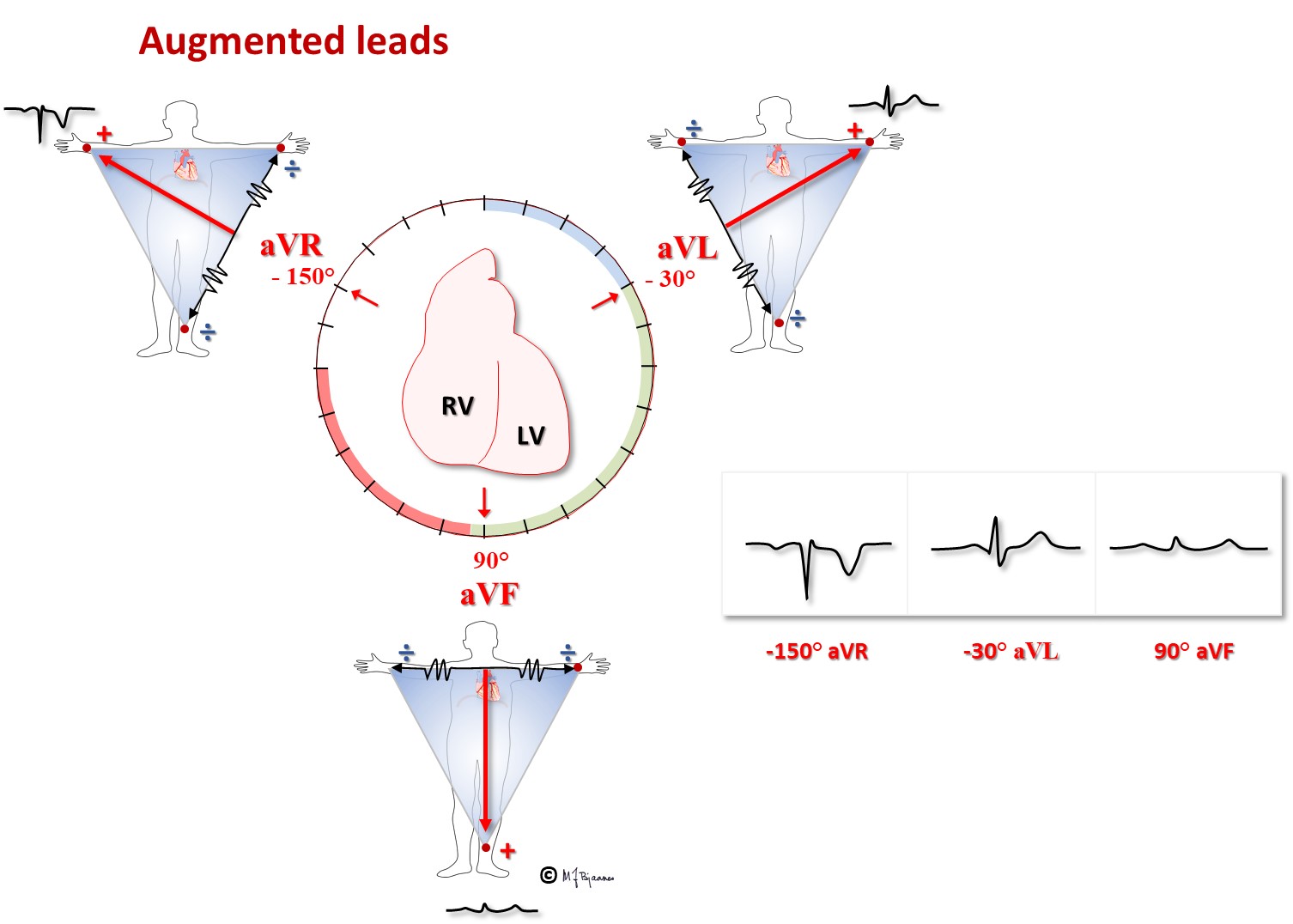
In elder literature the letters U and V were often interchanged (neuro or nevro, etc), and the new leads were named unipolar right (VR), left (VL) and foot (VF). Such a coupling, however, results in low amplitudes, so later on Goldberger changed the coupling, excluding the exploring anode from the central terminal, and thus measured the voltage of VR against VL and VF, VL against VR and VF, and VF against VR og VL. The amplitudes were now larger, and renamed ("a" for augmented): aVR, aVL and aVF. The precordial leads still use the original Wilson’s central terminal.
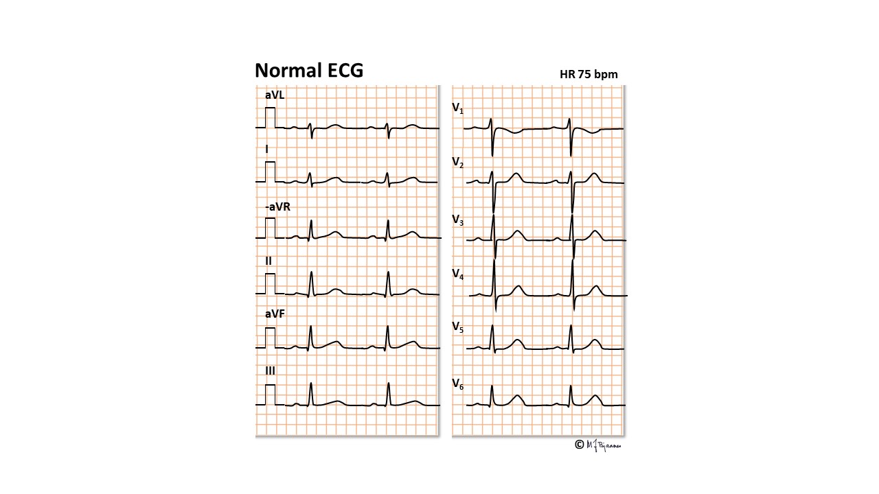
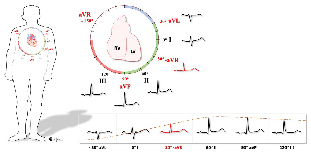
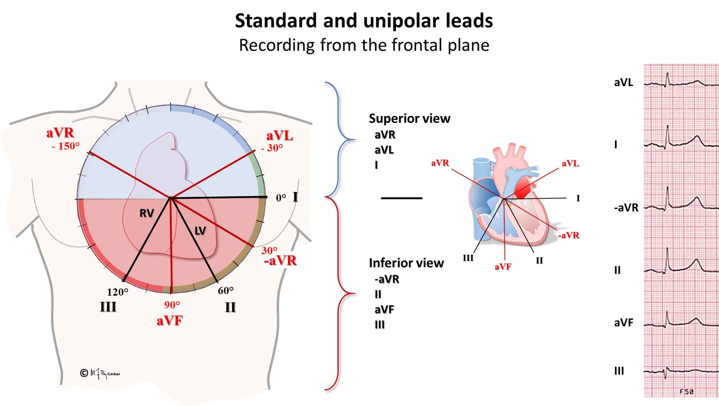
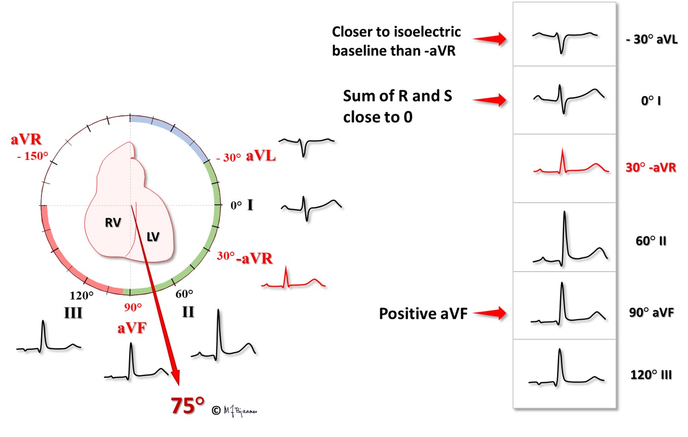
Regarding the three standard and three unipolar frontal plane leads, one deviates markedly from the other ones: aVR «looks at the heart» from above, from the right shoulder. The Spanish cardiologist Cabrera therefore reversed the coupling, and changed aVR to minus aVR (-aVR) within the recorder. Then the leads could be presented at 30° angles, from -30° to 120°: aVL - I - -aVR – II – aVF – III. Just like each of the precordial leads V1-V6 looks like an intermediate between the two adjacent neighbor leads, also the frontal plane leads are ordered similarly in the modern presentation panel. In this way, erroneous lead placement or coupling is more easily detected, and axis calculation is facilitated. Please note that all these six leads “view” the heart in the frontal plane.
Norwegian hospitals use the Cabrera presentation and a paper speed of 50 mm/s as their standard setup. Many distributors of ECG for general practitioners are, however, not aware of the benefit of the modern setup, and hence we still often see the old-fashioned sequence with I-II-III followed by aVR, aVL and aVF. Fortunately, reprogramming the machine is a simple task.
The 12 ECG leads register the cardiac electrical activity as seen from different angles in two planes.
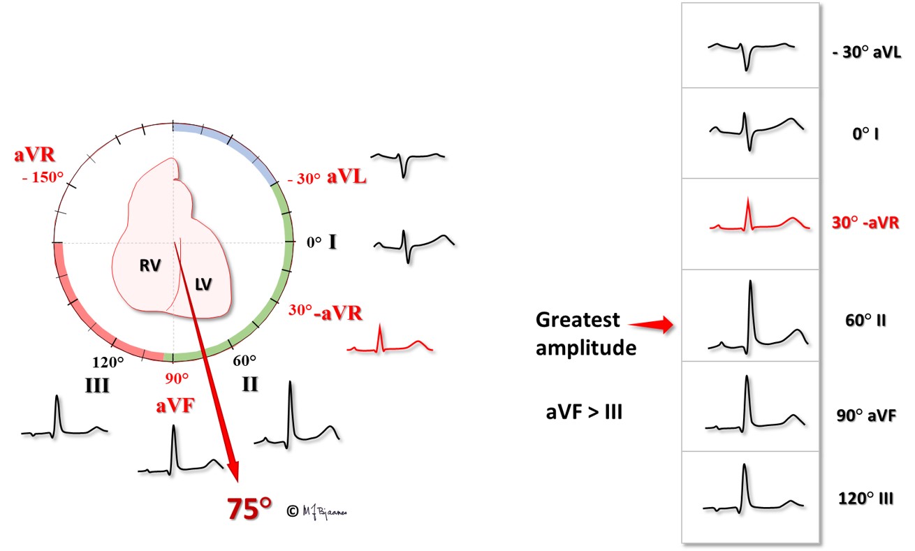
You may also start by finding a lead that is isoelectric (flat, or equal area under the positive and negative deflections). That lead must be perpendicular to the axis. In the example above, that is lead I. Then the axis must be either close to 90° (downward) or -90° (upward). Now look at aVF; it is positive, i.e. conduction is downward. Then we adjust according to the neighbor deflections: aVL is a little more isoelectric than –aVR, and again, we arrive at a QRS axis of 75°.
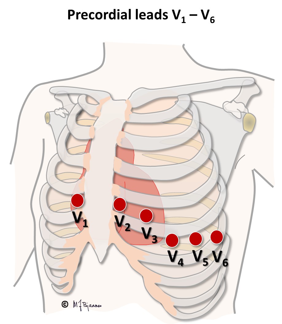
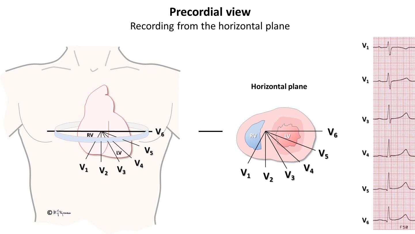
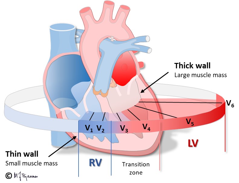
V1-V6 are placed in a row upon intercostal spaces from the sternal right side (above the right ventricle) to the left axilla (left ventricle), an almost horizontal plane. As the right ventricular wall is thin, and the left ventricular wall is thick, the main QRS amplitude will be directed away from V1 (rS) and gradually increase to its largest in V5-V6 (qR): this is called a smooth r-wave transition. Remember that R-waves reflect electrical forces that are directed toward an electrode, whereas S-waves reflect current directed away from the lead.
V1 and V2 are mainly influenced by the right ventricle, and V5 and V6 by the left. The transition zone is where rS changes to Rs (R>S), usually above the ventricular septum at V3-V4. Imagine you look at the heart from below: the horizontal heart axis is rotated clockwise if the transition zone is at V4-V6, and counterclockwise) in case the transition is at V1-V2.
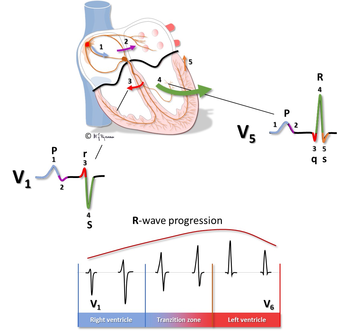
The 12 channels of the standard ECG are usually presented on two A4 sheet, the first with the standard leads according to Cabrera (aVL, I, -aVR, II, aVF and III), and the next sheet shows the precordials V1-V6. Again, note the smooth R-wave transition in both panels.